
Filter data in Numbers on iPad
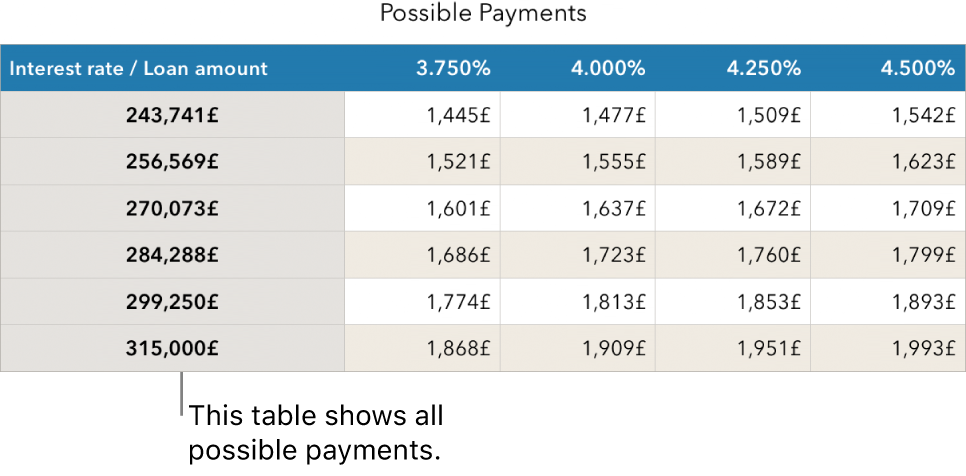
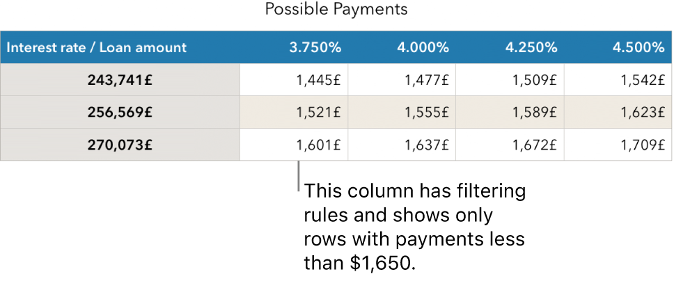
You can filter the data in a table to show only the data you want to see. For example, if you’re looking at a table of possible monthly mortgage payments for a loan with various interest rates, you can filter the table to show only the loans you can afford.
You filter data by creating rules that determine which rows in a table are visible. For example, you can create a filtering rule that shows rows that contain a number greater than a certain value or text that contains a certain word or, you can use Quick Filters to quickly show or hide rows.
Use Quick Filters
You can quickly show or hide rows that match a specific value in a column using Quick Filter. If you’re using Quick Filter in a pivot table, you can also hide (and show) groups in the Column and Row fields.
Go to the Numbers app
 on your iPad.
Open a spreadsheet, then select a column or cell.
If you want to use Quick Filters with a pivot table, select a header cell, row or column.
Tap
 or
or  at the bottom of the screen, then tap Quick Filter.
Select or de-select the check box for the data you want to show or hide.
Tip: If you are working with a large set of data and want to see only the items that are currently selected in the list, tap Show Selected.
When you’ve finished, tap anywhere on the sheet.
To see your Quick Filter rules, tap ![]() , then tap Filter.
, then tap Filter.
Create a filtering rule
You can create filtering rules based on the values in a column. Only rows with the specified values in that column appear. When you create a filtering rule for a pivot table, you can also create rules based on the fields.
Go to the Numbers app
on your iPad.Open a spreadsheet, tap the table, tap
 , then tap Filter.
Tap Add a Filter, then tap a column (or field) to filter by.
Tap the type of filter you want (for example, Text), then tap a rule (for example, “Starts with”).
You can also choose a Quick Filter.
Enter values for your rule — for example, if you select “Is not”, type text such as “Due by”.
Tap
 .
.To add another rule for the same column, tap Add a Rule, then choose a new filtering rule.
You can have multiple rules for a column — for example, show rows that have “yes” or “maybe” in Column C.
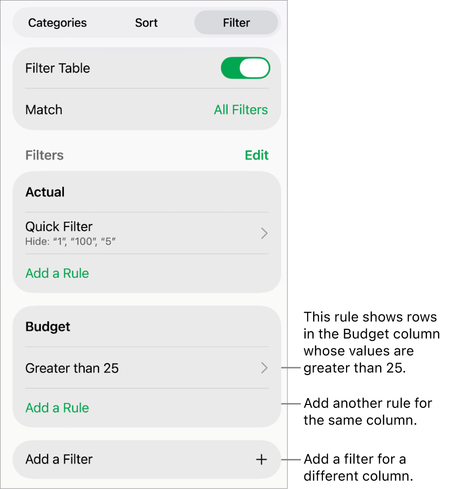
To add a filter to a different column, tap Add a Filter and choose another filtering rule.
In a table with multiple filtering rules, to show rows that match all filters or any filter, tap All Filters or Any Filter.
When you add rows to a filtered table, the cells are populated to meet the existing filtering rules.
Turn off filters or delete a rule
You can turn off all filters for a table without deleting them. You can turn them back on later if necessary. If you don’t need a filter, you can delete it.
Go to the Numbers app
on your iPad.Open a spreadsheet, tap the table, tap
, then tap Filter.Do either of the following:
Turn off all filters: Turn off Filter Table.
Delete a rule: Swipe left on a rule, then tap Delete. To delete a filter, delete all its rules.