Add or remove rows and columns in Numbers on iPhone
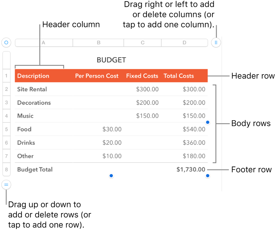
You can add, delete, and rearrange rows and columns in a table. There are three types of rows and columns:
Body rows and columns contain the table data.
Header rows and columns (if any) appear at the top and left side of the table. They usually have a different background color from the body rows, and they’re typically used to identify what the row or column contains. Data in header cells isn’t used in calculations, but the text in a header cell can be used in formulas to refer to the entire row or column. A table can have up to five header rows and five header columns.
You can freeze (or lock) header rows and columns so that they’re always visible when you scroll the spreadsheet.
Footer rows (if any) appear at the bottom of a table. A table can have up to five footer rows.

Add or remove rows and columns
Tap the table.
Do any of the following:
Add or delete a row or column at the edge of the table: Tap
 in the bottom-left corner of the table to add one row; drag
  down or up to add or delete multiple rows. Tap
  in the top-right corner of the table to add one column; drag
  to add or delete multiple columns. You can delete a row or column only if all of its cells are empty.
Insert a row or column within the table: Select an adjacent row or column (tap the row number or column letter), tap
 or
or  , then tap a placement option.
Insert multiple rows or columns within the table: Select a number of rows or columns—equal to the number you want to insert and adjacent to where you want to insert them—tap
 or
or  , then tap a placement option.
Delete a row or column within the table: Select the row or column, then tap Delete in the shortcut menu.
Add, remove, or freeze header rows and columns
Adding header rows, header columns, or footer rows converts existing rows or columns into headers or footers. For example, if you have data in the first row of a table and you add a header row, the first row is converted to a header row that contains the same data.
You can freeze header rows or columns so they’re always visible as you scroll the spreadsheet.
Tap the table, tap
 , tap Table, then tap Headers & Footer.
Do any of the following:
Add or delete headers and footers: Tap
 next to a header or footer category.
Freeze header rows or columns: Turn Freeze Rows or Freeze Columns on or off.
Hide or show rows and columns
Hiding rows or columns is useful if, for example, you need to use their data for formulas, but you don’t want the data to be visible.
Tap the table.
Do one of the following:
Hide rows or columns: Select one or more rows or columns to hide, tap
 or
or  , then tap an option.
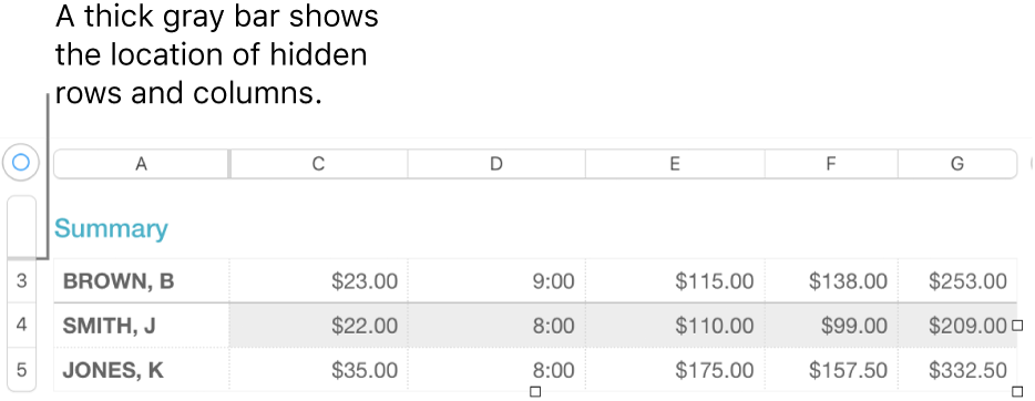
A gray bar appears between the column letters or row numbers to show where columns and rows are hidden.

Show hidden rows or columns: Tap any row number or column letter, tap
 or
or  , then tap Unhide All Rows or Unhide All Columns.
Display filtered rows
If you import a Numbers or Microsoft Excel spreadsheet with filtering turned on, some rows in your table may be hidden (or filtered). To display rows that are filtered out, you must turn off filtering.
Tap the table, tap
 in its top-left corner, then tap
  in the bottom-right corner of the screen.
Tap Turn Filters Off (if you don’t see Turn Filters Off, there’s no filtering).
To reapply the filtering criteria, tap Turn Filters On. You can’t add or edit filtering criteria on your iPhone or iPad.