Change how pivot table data is sorted, grouped and more in Numbers on iPhone
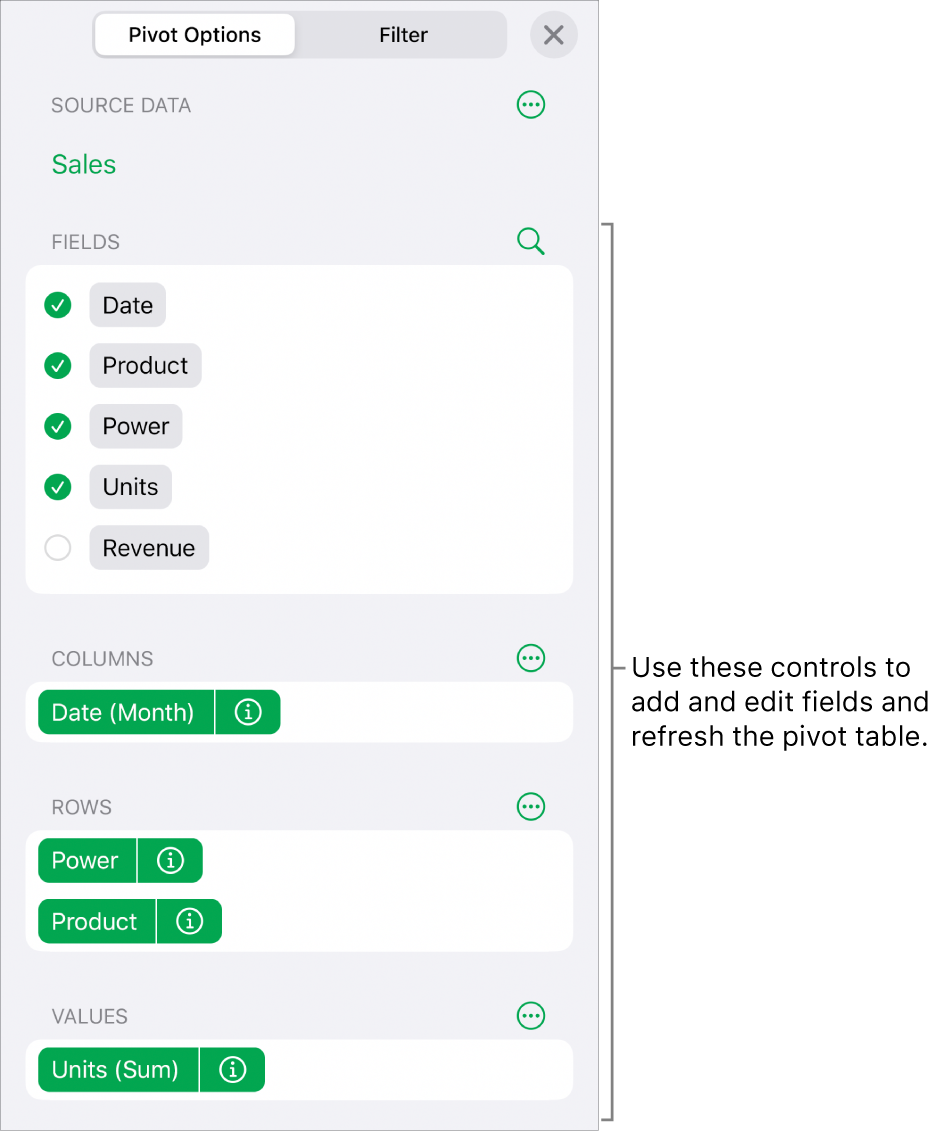
You can edit pivot table fields, including how they are sorted, grouped and calculated. You can also choose to repeat group labels and show and hide totals.
Tip: If you want to change the style or formatting for certain types of data in your pivot table (for example, Total rows), you can quickly select all data of the same type. Tap a cell you want to format, tap ![]() , then tap Select Similar Cells.
, then tap Select Similar Cells.

Change how Column and Row fields are sorted
You can change the way groups in a field are sorted in the table. For example, you can sort a group of students by their name in descending order (3, 2, 1…), or sort the group by their average grade in the class in ascending order (1, 2, 3…). You can also choose how to group dates, such as by year, year-month-day or day of week.
Select a pivot table.
Tap
 , tap Pivot Options, tap
  next to the Column or Row field you want to edit, then do any of the following:
Choose how to sort groups: Tap an option below Sort Groups By.
Sort values in ascending or descending order: Tap Order to choose between Ascending or Descending.
Choose how to group dates: Tap an option below Group By.
Repeat Column or Row group names
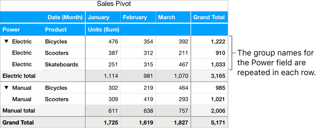
You can choose whether you want to repeat the group name labels for Column or Row fields in each column or row in the pivot table.
When there are multiple fields in the Column or Row section, you can repeat group names for all fields in that section (except the last field listed in that section). When there are multiple fields in the Values section, you can also repeat group names for each column or row where values appear.

Select a pivot table.
Tap
 , tap Pivot Options, tap
  next to the Column or Row field you want to repeat the labels for, then turn on Repeat Group Names.
Change how Value fields are displayed
Value fields use functions to summarise the data in pivot tables. You can choose from a list of functions, as well as change how the result is displayed. For example, you can calculate the sum of sales by an individual salesperson, then display the result as the percentage of total sales by the entire sales team.
Select a pivot table.
Tap
 , then tap Pivot Options.
Tap
 next to the Value field you want to change, then do any of the following:
Choose a new function: Tap Summarise By, then choose a function.
Change how the value is calculated: Tap an option below Show As. For example, you can show the result of the function as a percentage of the Grand Total, or as part of the Running Total for a Column or Row field.
If you choose Running Total In or % of Running Total In, you can choose which field is used to make that calculation.
If you have more than one Value field, you can also choose whether to show those fields as rows or columns. Tap ![]() next to Values, then tap Show Values as Rows or Show Values as Columns.
next to Values, then tap Show Values as Rows or Show Values as Columns.
Show or hide totals
When you add fields to a pivot table, Totals and Grand Totals are shown by default, but you can hide them.

Select a pivot table.
Tap
 , tap Pivot Options, then do any of the following:
Show or hide Total columns or rows: Tap
 next to the Column or Row field you want, then turn Show Total Columns or Show Total Rows on or off.
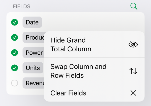
Show or hide Grand Total columns and rows: Tap
 next Columns or Rows, then choose Hide Grand Total Column or Hide Grand Total Row.
You can add filtering rules to change what data appears in the pivot table. See Filter data in Numbers on iPhone.