Intro to pivot tables in Numbers on iPad
You can create pivot tables to analyse any set of data, quickly group and summarise values and identify interesting patterns and trends.
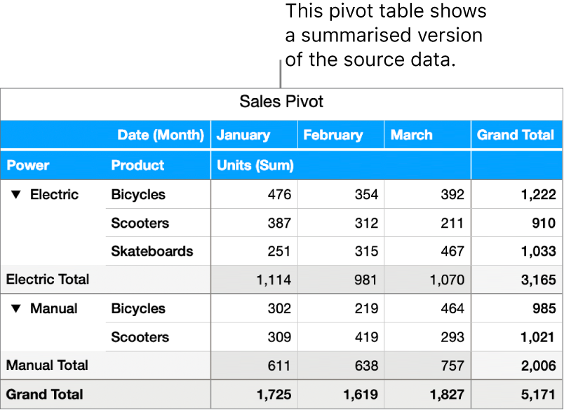
A pivot table can be created from a table or range of cells in a spreadsheet; the data used in those cells is your source data. The source data must contain at least one populated, non-header cell and can’t contain cells merged across adjacent rows. If you update the source data, you need to refresh the pivot table to see the changes. See Refresh a pivot table in Numbers on iPad.
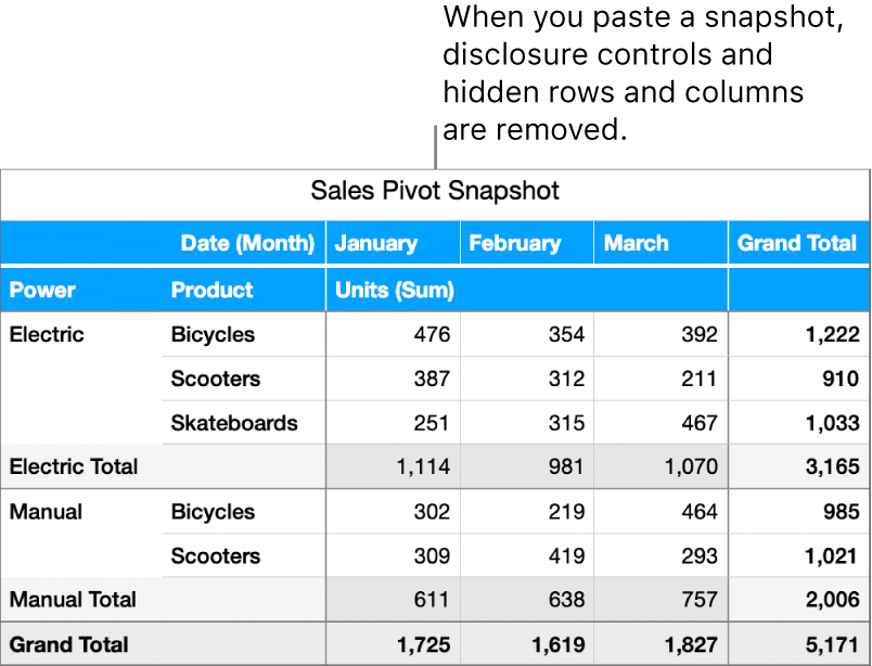
When you create a pivot table, you add fields that correspond with columns of data in your source data. Fields can be added to three sections — Columns, Rows and Values — and the placement and order of fields determine how your data is grouped in the pivot table. For example, if you place a field (Power) in the Rows section in the pivot table above, a row is added to the pivot table for each unique value (Electric and Manual) in the corresponding column in your source data. If you add another field (Product) to the Rows section, you create a hierarchy of rows, resulting in distinct groups of data (for example, electric bicycles and manual bicycles).
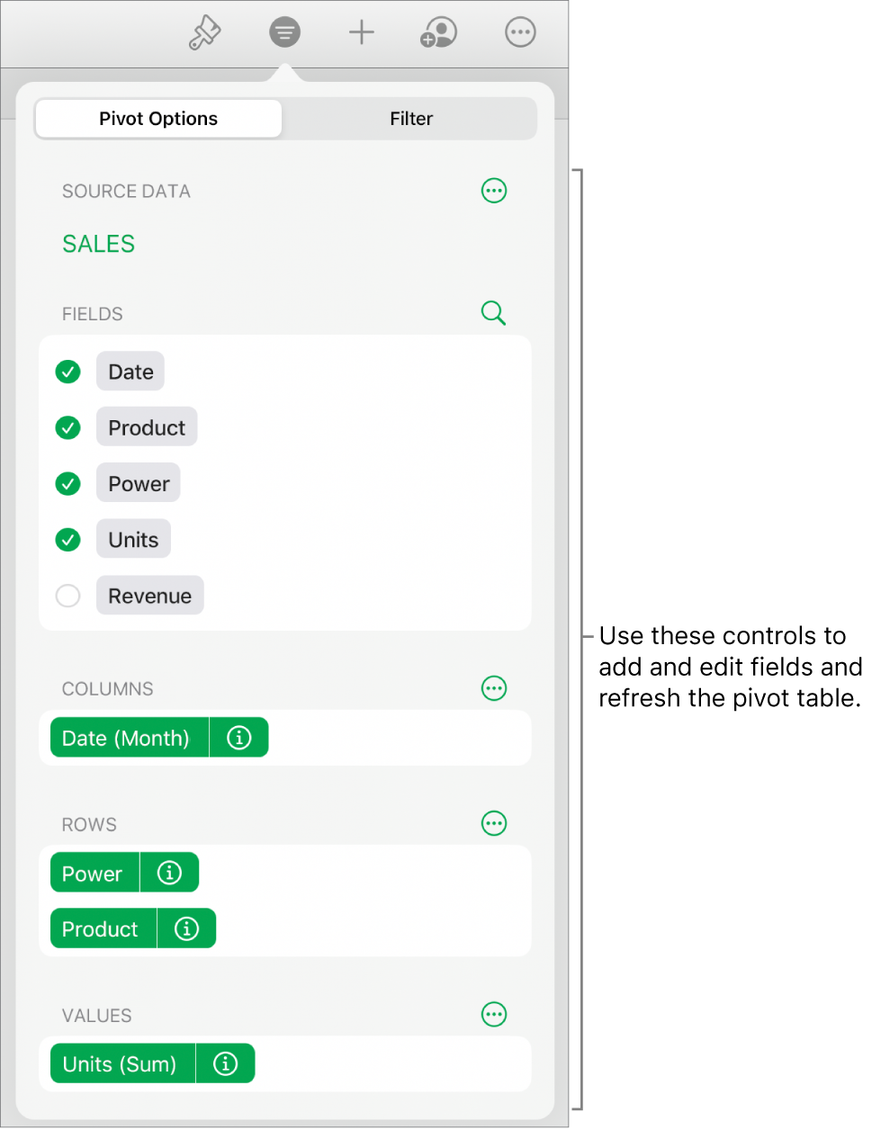
Value fields use functions, such as sum or average, to summarise data. You can change which function is used, how to display the results in the pivot table and whether you want to see Totals and Grand Totals.
To include only specific source data in the pivot table, you can use Quick Filters and create filtering rules. See Filter data in Numbers on iPad.
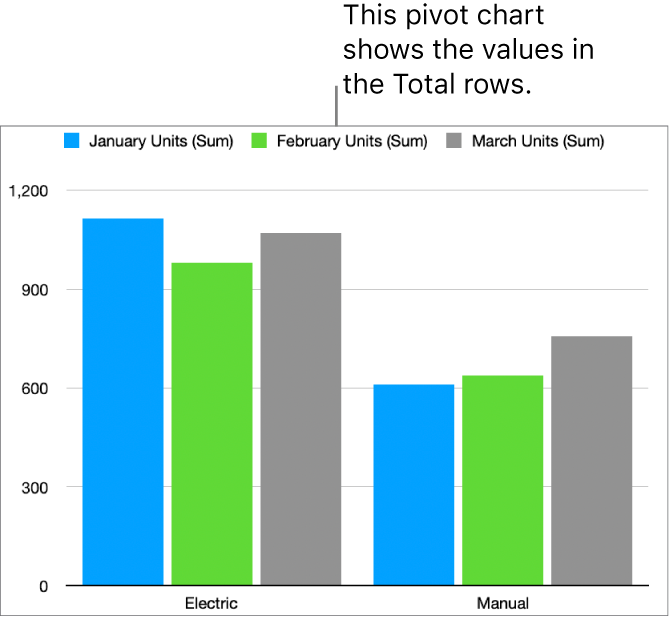
You can visualise trends in your pivot table by creating a chart. When you create a pivot chart, you can plot different data (such as Grand Totals) based on the cells you select. The pivot chart below displays the values in the Total rows (Electric and Manual) in the pivot table above. See Select cells in a pivot table to create a pivot chart.
You can also create a snapshot of your pivot table. The snapshot is a copy of your pivot table that is not affected by changes to the source data but has the same formatting as the pivot table. This is particularly useful for copying a pivot table to other apps, such as Pages or Notes. Using a snapshot is also a way to customise a pivot table; for example, you can use different labels or manually organise rows and columns.
You can import and export pivot tables to and from Excel. To learn more, see Import an Excel or text file into Numbers on iPad or Export to other file formats in Numbers on iPad.
Tip: You can also learn about pivot tables in the Pivot Table Basics template. With the spreadsheet manager in browse view, tap ![]() , then tap Pivot Table Basics in the Basic template category. Tap the tabs near the top of the template (Pivot Table Basics and Pivot Table Practice) to view the different sheets.
, then tap Pivot Table Basics in the Basic template category. Tap the tabs near the top of the template (Pivot Table Basics and Pivot Table Practice) to view the different sheets.
To get started with pivot tables, see any of the links below.