Add formulas to cells in Keynote for iCloud

You can create simple or complex arithmetic formulas using mathematical operators for addition (+), subtraction (-), multiplication (*), and division (/).

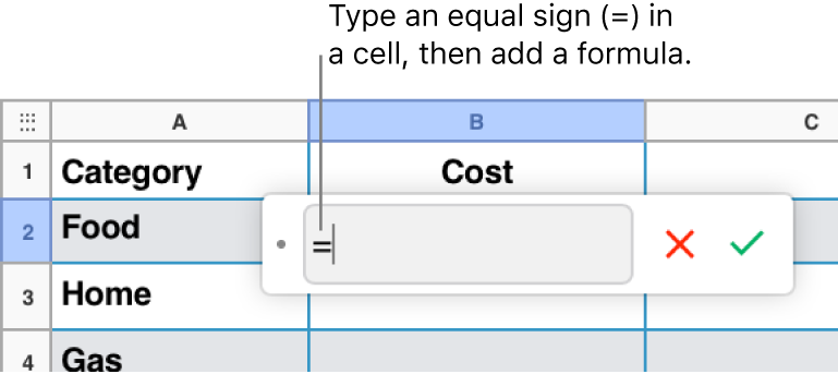
1. Click the cell where you want the result to appear, then enter the equal sign (=).

   The formula editor opens.

   

2. Enter a left parenthesis ( to begin your formula.

3. Click a cell to use as the first argument in your formula, or enter a value (for example, a number such as 0 or 5.20).

4. Enter an arithmetic operator (for example, +, -, *, or /), then either select a cell to use as the next argument in your formula, or enter a value.

5. Continue adding operators and arguments until your formula is complete.

6. Enter a right parenthesis ) to end your formula.

7. Press Return or click the Checkmark button in the formula editor when you’re done.

   If you click the Cancel button , you exit the current cell without saving the formula in it.

You can create a formula that uses comparison operators to check whether the values in two cells are equal, or if one value is greater or less than the other. To do this, you must set up a statement within a cell, for example A1 > A2, meaning the value in cell A1 is greater than the value in cell A2. The result of the comparison operator is expressed as “true” or “false.”

1. Click the cell where you want the comparison result to appear, then enter the equal sign (=).

   The formula editor opens.

   

2. Select a cell whose value you want to compare, or enter a value to compare.

3. Enter a comparison operator (>, >=, =, <>, <, or <=), then select a cell whose value you want to compare, or enter a value to compare.

4. Press Return or click the Checkmark button in the formula editor when you’re done.

   If you click the Cancel button , you exit the current cell without saving the formula in it.

There are predefined functions for applications including statistics, engineering, and finance, some of which retrieve information remotely via the internet. You can see the available functions in the Functions Browser, which appears in the Format sidebar on the right when you type an equal sign (=) in a table cell. The Functions Browser includes examples showing how the functions work, to help you choose one that suits your needs.

1. Click the cell where you want the result of the function to appear, then enter the equal sign (=).

   The formula editor opens, and the Functions Browser appears in the Format sidebar.

2. Enter the function name you want in the search field at the top of the Functions Browser, or browse the available functions, then double-click the name of the function you want.

   The function appears in the formula editor.

   

3. Click an argument within the function to select it.

   

4. Select the cells you want to include in the calculation by doing one of the following:

   • Add values in discontiguous cells: Click each cell you want to include.

   • Select a range of cells across multiple rows and columns: Drag across the range of cells you want to include.

   • Add the values of a single column or row: Click the column or row.

   The cell references appear in the formula editor.

5. Press Return or click the Checkmark button in the formula editor when you’re done.

   If you click the Cancel button , you exit the current cell without saving the formula in it.

You can quickly view the sum, average, minimum, maximum, and count for any column, row, or range of cells. (If the selection contains a mix of data types, such as text and numbers, or mixed formats, such as date and currency, some calculations aren’t provided.)

• Select the cells whose information you want to view.

  The results of the relevant calculations appear in the formula bar at the top of the sheet.

You can “freeze” row or column references in a formula so you can use the same formula elsewhere in your table without changing the cell references.

If you don’t preserve the row or column references, then if you move the formula (by cutting and pasting, or by adding new rows and columns), the references are adjusted relative to the formula’s new location.

1. Double-click the results cell with the formula you want to edit.

   The formula editor opens displaying the functions.

2. Click the triangle on the token representing the cell range you want to preserve.

3. Click Preserve Row or Preserve Column for the beginning or end addresses of the selected range.

   If you subsequently change the number of rows or columns in the table, or if you move the formula to a different cell, the preserved row or column references are adjusted.

4. Press Return or click the Checkmark button in the formula editor when you’re done.

   If you click the Cancel button , you exit the current cell without saving the formula in it.